Synthetic Replication of Bond Indices
4. März 2020 |
Disclaimer – The views and opinions expressed in this blog are those of the author and do not necessarily reflect the views of Scalable Capital Bank GmbH or its subsidiaries. Further information can be found at the end of this article.
In the last post in our series on fixed-income securities we have seen that investors might want to hold an ongoing exposure to a particular range of the yield curve. The problem with this is that individual bonds will change their time to maturity on an ongoing basis with the passage of time. Furthermore, they come with a fixed date of expiry where the investment itself is terminated. Individual bonds differ significantly from equities in this regard. While equities could be held infinitely long (except for company defaults or other reasons like stock buybacks), investors need to continuously adapt their bond portfolio if they want to have an investment that lasts forever. In order to relieve investors from the burden of continuously adapting their fixed-income portfolio, fixed-income ETFs usually follow some rollover logic such that ETFs become a convenient product that could be held for arbitrary investment horizons. Most fixed-income ETFs are either market-capitalisation-weighted, or they explicitly target a specific maturity range in some fixed-income market like, for example, US Treasuries with time to maturity between 7 and 10 years. In both cases, the ETF itself is a basket of individual fixed-income securities of different maturities, different coupon rates, and potentially also different issuers with different credit ratings.
In a previous post of this series we have already seen how varying interest rates can be translated into varying fixed-income security prices. For individual bonds, the price of the bond is just a deterministic function of interest rates and bond characteristics (cash-flow dates and cash-flow amounts). We have also seen how we can get a total return performance series by re-investing any coupon payments, and that the long-term total return performance actually might be increasing with increasing rates. Although increasing rates will cause the price of the fixed-income product to decline, re-investments of coupon payments at now higher interest rates might actually increase the total return of the security. As a next step, we now want to understand the impact of interest rate changes on bond ETFs, where each individual bond within the ETF portfolio comes with its own future cash-flows. In the case that the individual bonds stem from the same fixed-income market and have similar credit ratings each of them could be priced individually from the same yield curve. But instead of pricing each security individually and then aggregating individual security prices into an overall basket value, we can simply assume that the basket is just a single security with cash-flows equal to the aggregated series of all individual cash-flow series. Now the only additional complexity that remains for our bond ETF is the total return component introduced by the rollover strategy that defines rebalancing events within the basket and re-investments of coupon payments. This essentially boils down to the total return computation that we have already seen for individual fixed-income securities. However, we require one further assumption to simplify matters: we assume that there is no drain in portfolio value, neither during rebalancing events, nor elsewhere. Given that the ETF tracks fixed-income securities of a reasonably liquid market, transaction costs will usually not play a major role. What could be a significant cause of portfolio drain though is any loss in value due to deterioration of credit quality or defaults on promised cash-flows. The simplified index replication methodology that we are going to derive in the following will only work for bond indices that are approximately free of credit risks (e.g. US Treasuries or other bond indices with triple A rating). As we will see in the following sections, in a simplified setup without defaults and with all individual bonds relating to some common yield curve we can even remove complexities much further and still capture the main essence of the basket price trajectory. The only additional information we need for this is some average time to maturity that the bond basket uses as a target. Any other complexities like the exact composition of the basket, cash-flows, rollover strategy and coupon rates we will ignore, but we will nevertheless get a very accurate picture of how the bond ETF reacts to interest rate changes. Once we have a simplified reconstruction of a bond ETF, this will be beneficial in multiple ways:
Instead of relying on the true bond index basket the replication methodology does use one major simplification: it pretends that the whole basket only consists of a single zero-coupon bond with maturity equal to the average maturity of the true index basket. By matching maturities the zero-coupon bond is exposed approximately to the same part of the yield curve as the true underlying bond basket. And by only using a single zero-coupon bond we will not have to deal with any cumbersome cash-flow series and also not have to think about any re-investment of coupon payments. However, holding a single zero-coupon bond fixed over time would decrease its time to maturity on a daily basis and hence its time to maturity would eventually deviate significantly from the original basket. Therefore, instead of simply holding a single zero-coupon bond over time, we will rebalance on a daily basis, sell the zero-coupon bond after a holding period of one day, and buy again a new zero-coupon bond with time to maturity equal to the maturity target. Let denote the price of a bond in , the coupon payment at time , and the discount factor required to discount a payment of value 1 at time to its value in . Furthermore, let denote the value of a continuously compounding yield curve at time at maturity . Then the value of a zero-coupon bond can be computed by
One day into the future, the same bond will have a different value even if the yield curve itself did not change, simply because the time to maturity now will be smaller by one day. Hence, discounting now will occur at a different interest rate (the yield curve will be evaluated at maturity decreased by one day), and over a different remaining time to the final cash-flow (also decreased by one day). On the sale date the value of the zero-coupon bond will therefore be:
Since we do not have any cash-flows (e.g. coupon payments), the change in value between and will already represent a total return. Let denote the gross return, then we get:
Now we only need to aggregate all gross returns of the individual periods in order to get a replication of the bond index performance. With Python code, the computations can be done as follows:
zero_coupon_prices = np.exp((-1) * int_maturity * decimal_daily_yields)
zero_coupon_prices_after_1_day = np.exp((-1) * (int_maturity - 1 / 365) * decimal_daily_yields_maturity_minus_1_day)

# compute bond index returns
merged = pd.merge(zero_coupon_prices.shift(1), zero_coupon_prices_after_1_day, left_index=True, right_index=True)
daily_idx_rets = ((merged.iloc[:, 1] / merged.iloc[:, 0])).dropna()

# aggregate daily returns
daily_bond_idx = daily_idx_rets.cumprod()
Let us now check how accurate this replication methodology actually works despite the major simplifications that it uses. Therefore, we will compare synthetically created bond index trajectories for multiple different target maturities with historic trajectories of existing bond indices. For this analysis we will use US Treasury rates and US Treasury bond indices. A good source for US Treasury rates is the dataset of estimated US Treasury yield curves provided by The Federal Reserve Board.1 The dataset consists of daily parameter estimates of Svensson yield curve models applied to US Treasuries from 1961 to the present. Yields are quoted in terms of continuous compounding, and yield curves are estimated by imposing a functional form on forward rate curves (see Gurkaynak et al. 2006). Given the parameters over time, one can derive yields over time by converting forward curves into yield curves and evaluating these yield curves at the desired maturities over time. This dataset is particularly useful for our replication methodology because it does not only provide us with constant maturity rates over time (which are usually restricted to integer multiples of years, like e.g. maturity rates equal to 5 or 6 years). As can be seen from the formula above, for example, the computation of total index returns for target maturity 5 years will also involve the yield at maturity 5 years minus 1 day in order to compute the price of correctly. Using instead of for the computation of would actually lead to surprisingly different results. This is the first thing that we want to analyse in further details with the data at hand. Therefore, we will compare synthetically computed bond indices with target maturity 5 years, once using correct interest rates (), and once using as an approximation instead. Both rates are shown in Figure 1.
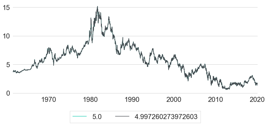
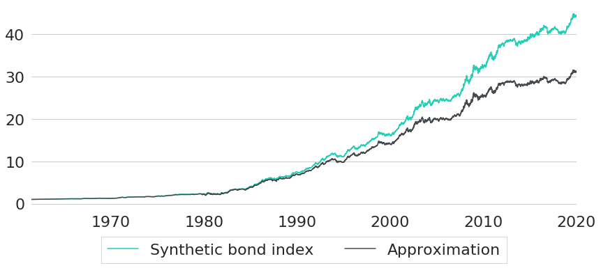
As we can see, yields for both maturities are basically indistinguishably close together. This is not really surprising, as both maturities differ only by a single day. However, even though we do not see any significant difference between both maturities, they will still lead to a surprisingly different synthetic index performance as shown in Figure 2. Using the true maturities, shifted by one day at time , gives the turquoise performance, while the approximation based on is shown in grey. For this sample, the difference in annualised return actually exceeds 0.5%.
As can be seen from this analysis, being precise with regards to the maturity chosen for discounting is quite important. In this regard, it is a nice feature of our interest rate data that we can evaluate yield curves at any arbitrary maturity. If we had used CMT rates instead, we would have to think about a sufficiently good approximation method for first (e.g. through interpolation of given CMT rates).
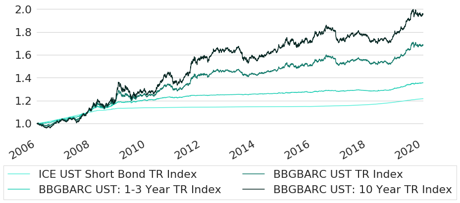
As a next step, let us now pick some existing bond indices that we want to replicate. Thereby we will pick the indices in such a way that all of them are targeting different sections of the yield curve (i.e. they have different average times to maturity). The indices we have picked, together with their Bloomberg tickers, are the following:
The indices have been sorted according to increasing average time to maturity. Data is from Bloomberg and shown in Figure 3. The first date that data for all indices is available is December 12th, 2005 due to a rather short history for the ICE UST Index. We cut off all data before that date and normalise it such that all indices start at value equal to 1 at this date.
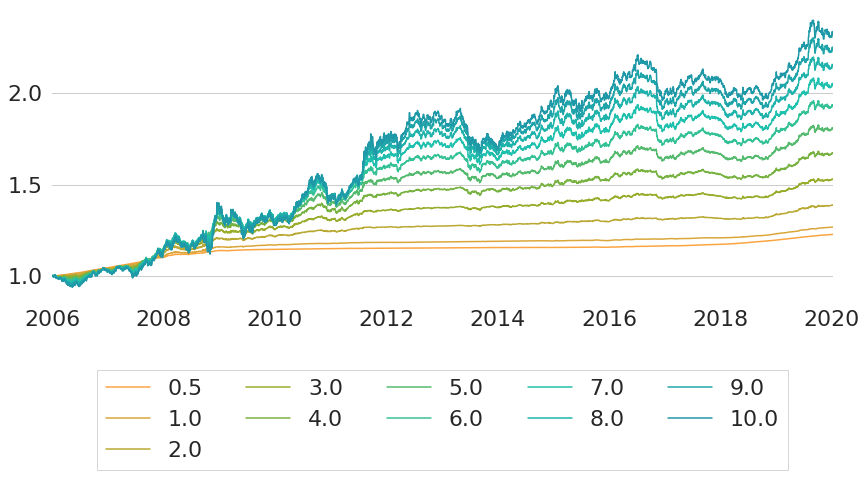
For the same time period we now generate synthetic bond index data for multiple maturities. Selected maturities comprise maturities for each full year from 1 year to 10 years, extended at the short end by a maturity of half a year. The synthetic bond index trajectories that we get are shown in Figure 4.
The maturities of the synthetic bond indices so far have been selected rather detached from the actual average maturities and durations of the existing bond indices. One reason for this is that these metrics will vary over time for every index and hence there is not a single correct constant target maturity anyway. Obviously, this is a point that one could further elaborate on in order to improve the replication of a given index. We will not further fine-tune this calibration parameter, however, for two reasons. First, even without exactly matching the target maturity on each single day the results will be sufficiently close to serve as proof of concept for the replication methodology. Second, in most of the subsequent analyses where we will use this methodology the aim will not be to replicate some given index as closely as possible, but rather to gain a general understanding into different yield curve exposures. In case that some of the synthetic indices actually seems to be a worthwhile investment that should be implemented, one either needs to select a closely matching existing index as an investment vehicle, or one could build a closely matching real world strategy on its own.
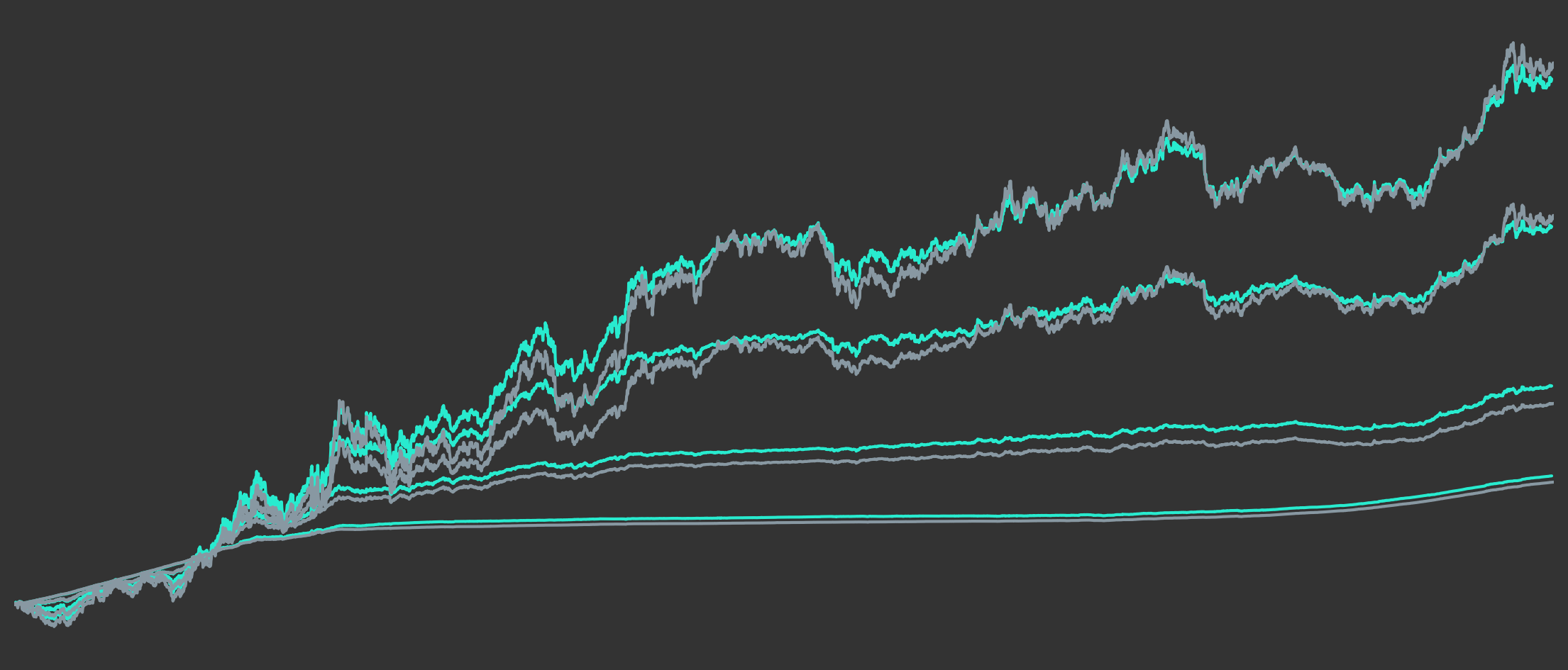
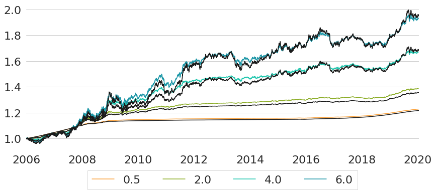
Figure 5 shows the performance of the existing indices compared to a subset of the synthetically constructed indices. The synthetic indices have been chosen such that they provide a good fit to the existing indices in terms of overall return of the full investment period. As we can see from the chart, for each of the existing indices we have a rather closely matching synthetic counterpart.
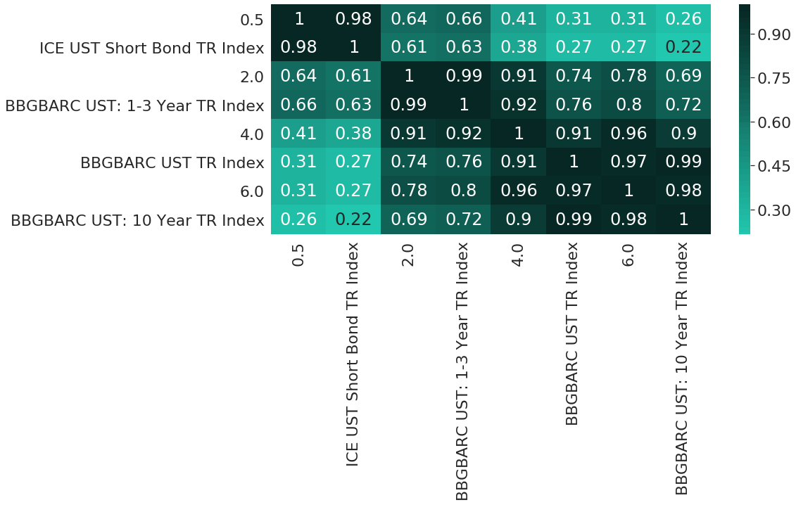
Only visually analysing performance charts can actually be misleading in many situations. Hence, let us now further validate the adequacy of the synthetic replications through a couple of other perspectives on the data. First, Figure 6 shows the correlation matrix for weekly returns of all 8 performance series. Of particular interest for us is the pairwise block-diagonal of the correlation matrix, as existing and synthetic indices are sorted in matching pairs. From the first block diagonal we can see that ICE US Treasury Short Bond TR Index and the synthetic index with target maturity 0.5 years have an almost perfect correlation with value equal to 0.98. The same also holds for both the pair involving the Bloomberg Barclays US Treasury 1-3 Year TR Index, as well as the pair for the Bloomberg Barclays US Government 10 Year Term TR Index. Only for the case of the Bloomberg Barclays US Treasury TR Unhedged USD is the correlation slightly lower with value equal to 0.91.
As a second validation method we also take a look at risk-return metrics of both existing and synthetic indices. In Figure 7 we can see annualised return and annualised volatility for each of the existing indices in turquoise, compared to all synthetic indices that we computed in dark grey. Figure 8 shows the same comparison, only with risk measured in terms of maximum drawdown instead of annualised volatility. In both charts we can see that the two less risky existing indices can be replicated pretty well in terms of both risk and return. Even though their points do not perfectly overlap with the corresponding points of the synthetic indices, they still are very close to the risk-return frontier that we would get by creating synthetic indices on an even finer target maturity grid. In other words, if we just fine-tuned the target maturities a bit better, then we could find an almost perfect replication for the existing indices.
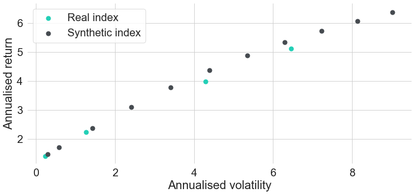
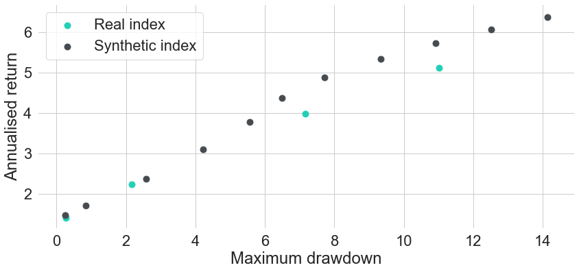
For the two existing indices with longer durations the story is a bit different. Both turquoise points seem to lie slightly below the risk-return frontier spanned by the synthetic indices. Hence, no matter how exactly we choose a single constant target maturity, we will never be able to replicate these indices exactly. In order to match their performance even closer, we could replicate their sensitivity to interest rates more precisely. One simple way of doing this is by allowing for varying target maturities over time in the construction methodology, because real indices usually never have fully constant average durations over time. As long as there is no significant drain in the portfolio value (e.g. from defaults) and all underlying securities can be priced from a single yield curve, the synthetic construction methodology is able to replicate real index prices pretty well.
Gurkaynak, Refet. S., Sack, Brian, and Wright, Jonathan H. (2006), The U.S. Treasury Yield Curve: 1961 to the Present, Federal Reserve Board Finance and Economics Discussion Series.
1: The U.S. Treasury Yield Curve of The Federal Reserve Board: https://www.federalreserve.gov/pubs/feds/2006/200628/200628abs.html. The same dataset can also be accessed more conveniently through Quandl: https://www.quandl.com/data/FED/PARAMS.
Disclaimer – The views and opinions expressed in this blog are those of the author and do not necessarily reflect the views of Scalable Capital Bank GmbH, its subsidiaries or its employees ("Scalable Capital", "we"). The content is provided to you solely for informational purposes and does not constitute, and should not be construed as, an offer or a solicitation of an offer, advice or recommendation to purchase any securities or other financial instruments. Any representation is for illustrative purposes only and is not representative of any Scalable Capital product or investment strategy. The academic concepts set forth herein are derived from sources believed by the author and Scalable Capital to be reliable and have no connection with the financial services offered by Scalable Capital. Past performance and forward-looking statements are not reliable indicators of future performance. The return may rise or fall as a result of currency fluctuations. Please refer to our risk information.
Risikohinweis – Die Kapitalanlage ist mit Risiken verbunden und kann zum Verlust des eingesetzten Vermögens führen. Weder vergangene Wertentwicklungen noch Prognosen haben eine verlässliche Aussagekraft über zukünftige Wertentwicklungen. Wir erbringen keine Anlage-, Rechts- und/oder Steuerberatung. Sollte diese Website Informationen über den Kapitalmarkt, Finanzinstrumente und/oder sonstige für die Kapitalanlage relevante Themen enthalten, so dienen diese Informationen ausschließlich der allgemeinen Erläuterung der von Unternehmen unserer Unternehmensgruppe erbrachten Wertpapierdienstleistungen. Bitte lesen Sie auch unsere Risikohinweise und Nutzungsbedingungen.