Trade Cost Optimisation
May 8, 2019 |
Disclaimer – The views and opinions expressed in this blog are those of the author and do not necessarily reflect the views of Scalable Capital Bank GmbH or its subsidiaries. Further information can be found at the end of this article.
Investors usually face a multi-objective optimisation problem. The main objective is to find the optimal portfolio for investing. Besides that, a second objective is to implement this optimal portfolio allocation in a cost-efficient manner.
Let us assume that we always trigger trading if the distance of our current portfolio from a given ideal portfolio is too large1. One way to measure distance between portfolios is turnover, , which is defined as the sum of the absolute distances of the portfolio weights of each asset scaled by one-half to obtain a measure in (see Section 3 for a formal definition). In the following, we will use as the trading trigger. This means that we trigger a trading event whenever the distance of the current weight, , to the ideal weight, , is larger than . A trade cost optimisation is used to determine new portfolio weights which are closer to the ideal portfolio weights than the current weights, but cheaper to accomplish than a full rebalancing to the ideal portfolio. Quite generally speaking, two implementation strategies are possible. First, the portfolio optimisation and the trade cost optimisation could be done in a joint optimisation step (see for example Mansini, Ogryczak and Speranza (2014) for a literature overview). And second, a two-step approach where the portfolio optimisation delivering an ideal weight vector, , for the portfolio is done in a first step, while trade costs are optimised only in a second step. The original ideal weight vector hence will be adapted by the trade cost optimisation, leading to a slightly different weight vector . We will focus on the second approach as it comes with two advantages. From a mathematical point of view it is much easier to implement. In addition to that, having trade cost optimisation and portfolio optimisation independent from each other allows one to combine the trade cost optimisation flexibly with any potential portfolio strategy. Whether the ideal weights are decided by an investment committee or obtained from a dynamic portfolio optimisation strategy, the trade cost optimisation approach can be applied in both cases.
Any trade cost optimisation needs to deal with a trade-off between cost efficiency and optimality of the new portfolio. One way to balance this trade-off is by defining a maximum acceptable distance to the ideal portfolio weights. This way only portfolio weight vectors with a distance less than the threshold become valid solutions in the optimisation problem. The closer this threshold is to zero, the less freedom the trade cost optimisation gets. Portfolio weights will be closer to the original target and hence "more optimal", but with less reductions in trading costs. Using such a threshold, a trade cost optimisation can be achieved by minimising the costs while keeping the distance to the ideal portfolio within bounds, i.e.,
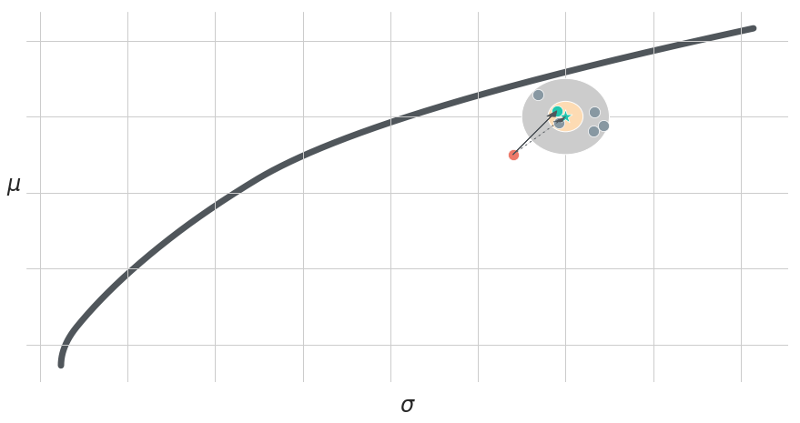
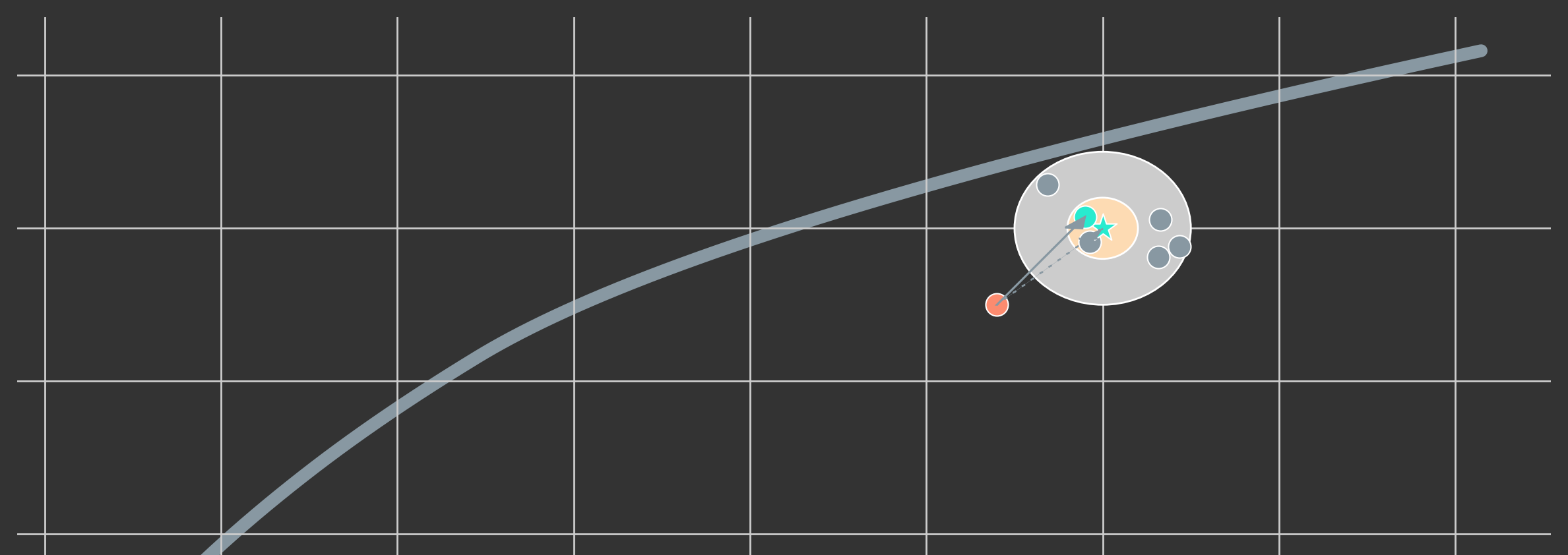
where are the costs to trade from to and is the turnover distance of the post-trade weights, , to the ideal weights, . An illustration of this approach is shown in Figure 1. While distances are actually measured in terms of portfolio weights, individual portfolios are represented in terms of risk and return in a --chart. The star represents the ideal weight of a hypothetical portfolio strategy and the outer circle around it visualises the area in which no trading is triggered. Only portfolios outside of this area exceed the threshold and need to be traded. The arrow represents the trading to the new weights instead of trading to the ideal weights (dashed arrow). Moreover, the inner circle represents the area into which the trade cost optimisation has to move in a trade-cost-efficient manner.
A second animated graphic (Figure 2) gives a visual impression of the trading behaviour of such a trade cost optimisation:
The more reduction of the distance to the ideal weight is enforced (represented as a bar in the lower left plot), the more trades need to be executed. The increase in trading costs is shown as a bar in the lower right plot of Figure 2, where the orange part represents fixed costs and the dark blue part variable costs. Fixed costs are for example fees which are charged per traded asset and variable costs can either be explicit fees per traded volume or implicit costs, like bid-ask-spreads, that are proportional to the traded volume. A typical fee structure for a retail investor using an online broker could be a fixed amount per executed order of $5.00 and a variable cost depending on the trade volume, e.g., 0.25% of the traded volume. This exemplary cost structure will be assumed in the following.
Moreover, the central part of Figure 2 shows in which assets buys (green) and sells (red) are proposed by the trade cost optimisation. The light green and light red part represent the weight distances from the ideal weights that the trade cost optimisation decided not to trade. The frames show the final post-trade-cost-optimisation portfolio weights.
To demonstrate the benefits of trade cost optimisation we now show achievable cost reductions for an exemplary systematic portfolio strategy. The strategy is taken from Portfolio Visualizer2, where the relative strength momentum strategy (Faber 2010) is applied for a US investor rotating across asset classes using the following ETFs: SHY, TLT, RWR, IWM, IWB, GLD, EFA, EEM, DBC. We use total return data from Bloomberg for the ETFs and for simplicity assume that all ETFs are accumulating their distributions so that there is no need to manually re-invest cash-flows in between. On a daily basis, we compute yearly returns (252 trading days) for every asset and invest into the top 5 performing assets equally weighted. In addition, we apply a regularisation step on daily ideal portfolio weights in order to reduce noise and to be less sensitive to effects like timing luck3. This regularisation step simply applies a moving-window (21 trading days) sample mean to daily portfolio weights from relative strength momentum indicators. This way portfolio weights cannot dramatically change from one day to the next anymore and hence become more smooth over time.
The trade cost optimisation in use relies on two key tuning parameters:
The turnover distance which needs to be exceeded such that we trigger a trading event and the turnover distance which is accepted directly after trading. The second parameter basically determines the tolerance in which the trade cost optimisation is allowed to operate. It controls the precision to which the optimal portfolio weights will be achieved after application of the trade cost optimisation. Setting enforces the trade cost optimisation to fully trade towards the ideal weights and, e.g., means that the trade cost optimisation has to reduce the turnover distance to the ideal weight until it is smaller or equal to half the turnover trigger. The trade cost optimisation is doing this in a cost-efficient way. A graphical illustration of the trade cost optimisation mechanism was already presented in Figure 2 for an example trade event.
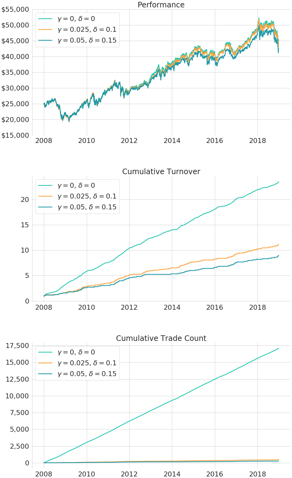
In Figure 3, we present the results for a backtest from Jan-2008 to Dec-2018 with an initial portfolio value of $25,000. Three different implementation strategies are considered: As benchmark case we consider the strategy without any trade cost optimisation (, ), i.e., we trade on a daily basis to the ideal weights. The two other strategies use the trade cost optimisation with parameter settings , and , . In all three cases we assume that fractional dealing is allowed. Results under a no-fractional-dealing condition are presented in Section 3.4.
In the top plot of Figure 3 we can see that the performance of the three settings is almost indistinguishable. Looking at the middle plot in Figure 3 for the cumulative turnover and the lower plot for the cumulative trade count it becomes clear that the trade cost optimisation can reduce trading costs to a huge extent. In particular, aggregate trade count, i.e. the number of executed trades, can be reduced significantly, but trading volume measured in terms of turnover is also reduced. At the same time the overall performance of the portfolio strategy does not change significantly and there is no systematic bias visible. Measured in terms of average daily turnover distance to the ideal weights for , the distance is 5.94% while it is 9.59% for , . This explains why it is almost impossible to visually distinguish the three cumulative performance graphs shown in the top plot of Figure 3.
The reductions in trading costs are indeed remarkable: The annualised turnover is reduced from 1.96 by 52.64% to 0.93 (by 61.92% to 0.75) for , (, ). The cost-efficiency gain is even more pronounced for the annualised trade count, which is reduced from 1,422 to 40 (24) trades per year, i.e., by 97.16% and 98.34% respectively. This means that the studied momentum strategy, which in the backtest has a turnover of almost 200% per year, can be implemented with an average of only 24 trades per year and the resulting portfolio allocations, and hence also the performance, is almost the same as the original strategy.
In the following, we will present technical details and mathematical derivations necessary to implement the trade cost optimisation. Readers not interested in those technical details are encouraged to directly jump to either Section 3.4, which contains the backtest results with a no-fractional-dealing condition, or to continue reading with the concluding remarks in Section 4.
Section 3 is organised as follows. In Section 3.1 we introduce measures for the distance of two portfolio weight vectors and explain the relation of those distances to different types of transaction costs. Moreover, we give a mathematical formulation of a no-fractional-dealing condition. Section 3.2 contains the mathematical formulation of the trade cost optimisation problem and in Section 3.3 we provide derivations in order to transform the trade cost optimisation problem into a mixed integer linear program (MILP) for which standard solvers exist. Finally, in Section 3.4 we show simulation results for the previously studied momentum strategy but under consideration of a no-fractional-dealing condition.
For simplicity, we restrict ourselves to the case of an existing portfolio with no deposits and assets. Our hypothetical investor intends to switch from one portfolio weight vector to another weight vector in a trade-cost-efficient manner.
Measuring the Distance Between Weight Vectors
The distance between two portfolio weight vectors and can be measured with different metrics:
where is the indicator function which is equal to one if is true and zero otherwise.
2. Trading volume
Note that all three distances are symmetric.
Measuring Transaction Costs
Trading from to comes at a cost. W.l.o.g. let the cash asset have index . It is used as a residual asset with target weight zero. Different types of costs can be represented in terms of weight distances4.
where denotes the total value of the portfolio.
3. Total costs
Portfolio Volumes, Weights and Fractional Dealing
For retail investors fractional dealing is often not possible. This implies that trade-cost efficient implementations need to handle integer constraints. If the price of asset is given by and the number of volumes invested in asset by , the total value of the portfolio can be computed as
and the portfolio weight for asset is given by . If fractional dealing is allowed, we have , whereas with no-fractional-dealing condition applies for all assets except cash ().
As explained in Section 1, a straightforward setup for a trade cost optimisation is to minimise the total costs under some constraint on the distance to the ideal portfolio weight. A trade event is triggered whenever . However, if the trading trigger is reached, we do not want to fully trade to our ideal weight and spend costs . Instead, the trade cost optimisation should deliver a new weight vector, , with minimum trading costs, but sufficiently close to the ideal weight vector (the maximum allowed distance is , with ).
In mathematical terms, the optimisation problem can be written as
where we use the notation and for column vectors of zeros and ones, respectively. Besides the already discussed turnover restriction, we added the standard portfolio budget constraint and a no-short-selling restriction. For simplicity, we also assume that trading costs are not directly deducted from the portfolio but externally charged, for example on a monthly basis from a reference bank account.
Standard solvers for convex problems are not well suited for such a problem as the and contain the absolute value function and even the absolute value function within the indicator function. Therefore, we will now show how the optimisation problem can be linearised using an augmentation technique to obtain a mixed integer linear program (MILP) which can be easily solved using standard software packages for numerical optimisation (see for example Roncalli (2013) where such an augmentation is also applied for quadratic programs).
For let be the current weight invested in asset and be the future, i.e., after-optimisation weight of asset . By introducing appropriate auxiliary variables and for each asset respectively, we can obtain
Without further constraints, we could find infinitely many combinations of and that fulfil this equation. However, if we impose the additional constraint , i.e., at least one of the variables or is necessarily equal to zero, and are uniquely defined and we can write
can then be interpreted as the excess weight of the final weight with regards to the initial portfolio weight . In other words: It measures how much the individual asset weight is increased. Similarly, represents a decrease in the weight of asset .
We can now re-write the variable costs as a linear function in the vectors and as
In a similar way, we also linearise the turnover distance between and by enforcing the identity
with the auxiliary variables and . Under the condition , we get
We can now re-write the optimisation constraint as a linear constraint in the vectors and
The fixed costs additionally contain an indicator function. Therefore, we need to add further binary auxiliary variables , for . Via inequality constraints, we will force the binary variable to be an indicator variable which is equal to one if and only if we trade asset . Let , and consider the inequality
If the inequality is fulfilled, it guarantees that when and when . Like the variable costs, we can re-write these constraints in terms of and as linear functions. Moreover, we can now also write the fixed costs as a linear function in
Note that, due to technical reasons, we have to assume a minimum trade size per asset of such that holds, i.e., either or .
Putting things together, we obtain the optimisation problem
where is a vector and denotes the Hadamard product.
The Non-Linear Constraints and
The non-linear constraints and can be indirectly integrated. Lets skip the non-linear constraints for a moment. Assume solves the new (without and constraints) optimisation problem. Then w.l.o.g.
Define the new variables (for ):
It holds
with for . Similarly, we can construct variables and with and . At the same time it holds
i.e., solves the original problem, including the non-linear constraints and as well as the turnover maximum constraint.
The Trade Cost Optimisation Problem as Mixed Integer Linear Program (MILP)
Having shown how to get rid of the non-linear constraint, we can write our optimisation problem as a mixed integer linear program (MILP) with linear (in-)equality constraints
with appropriately selected matrices and vectors , , , and .
Integrating a No-Fractional-Dealing Condition into the Trade Cost Optimisation Problem
Using the identity , we can obtain post-trade volumes and corresponding buy and sell volumes as
Defining and , we obtain the trade cost optimisation with no-fractional-dealing condition as
where and , with . Moreover, , denote the number of rows of and , respectively and denotes the Kronecker product.
We rerun our momentum strategy backtest to see the impact of a no-fractional-dealing condition applied to all nine ETFs. Table 1 summarises the results. We can see that, even with a no-fractional-dealing condition, the trade cost optimisation is capable of keeping the average daily turnover distances to the ideal portfolio on a similar level. At the same time the annual turnovers are almost unchanged, but we observe mildly increasing trade costs in terms of an increase in the annual trade counts. This means that even under the more complex integer constraint of a no-fractional-dealing condition, the trade cost optimisation approach allows us to implement the momentum strategy in a cost-efficient way while keeping the distance to the ideal portfolio within certain bounds.
Parameters & metrics |
No trade cost optimisation |
Setting 1 with fractional dealing |
Setting 1 without fractional dealing |
Setting 2 with fractional dealing |
Setting 2 without fractional dealing |
|---|---|---|---|---|---|
|
|
|
|
|
|
Average in % |
0.00 |
5.94 |
6.01 |
9.59 |
9.37 |
Annualised turnover |
1.96 |
0.93 |
0.98 |
0.75 |
0.73 |
Annualised trade count |
1422.25 |
40.33 |
51.75 |
23.67 |
27.42 |
In this blog article we introduced an efficient and flexible trade cost optimisation approach. It can be combined with every portfolio optimisation strategy in a two-step setup. Tuning of the optimisation parameters allows customisation of the trade cost optimisation to individual cost structures and requirements with regards to proximity of realised weights to ideal weights.
We demonstrated the benefits of the presented trade cost optimisation approach in a backtest by showing that a momentum strategy with a yearly turnover of 200% can be implemented with an average of only 24 trades per year. The main challenge in the technical implementation of the trade cost optimisation is the reformulation of the optimisation problem as a mixed integer linear program (MILP). Our derivation of a MILP representation allows a straightforward implementation in every standard software package for numerical optimisation.
Faber, M. (2010), Relative Strength Strategies for Investing, Available at SSRN: http://dx.doi.org/10.2139/ssrn.1585517.
Hoffstein, C., Sibears, D. J. and Faber, N. (2019), Rebalance Timing Luck: The Difference Between Hired and Fired, The Journal of Index Investing, https://doi.org/10.3905/jii.2019.1.070.
Mansini, R., Ogryczak, W. and Speranza, M. G. (2014), Twenty years of linear programming based portfolio optimization, European Journal of Operational Research, 234 (2), pp. 518-535.
Roncalli, T. (2013), Introduction to Risk Parity and Budgeting, Chapman & Hall/CRC Financial Mathematics Series.
1: As an alternative, we could also use a calendar-based trading trigger, like monthly or weekly.
2: https://www.portfoliovisualizer.com/examples
3: See Hoffstein, Sibears and Faber (2019) and https://blog.thinknewfound.com/2018/01/quantifying-timing-luck/ for a discussion of timing luck.
4: We use the notation and , etc., if the first index (w.l.o.g. cash) is skipped in the distance measure.
Disclaimer – The views and opinions expressed in this blog are those of the author and do not necessarily reflect the views of Scalable Capital Bank GmbH, its subsidiaries or its employees ("Scalable Capital", "we"). The content is provided to you solely for informational purposes and does not constitute, and should not be construed as, an offer or a solicitation of an offer, advice or recommendation to purchase any securities or other financial instruments. Any representation is for illustrative purposes only and is not representative of any Scalable Capital product or investment strategy. The academic concepts set forth herein are derived from sources believed by the author and Scalable Capital to be reliable and have no connection with the financial services offered by Scalable Capital. Past performance and forward-looking statements are not reliable indicators of future performance. The return may rise or fall as a result of currency fluctuations. Please refer to our risk information.
Risk Disclaimer – There are risks associated with investing. The value of your investment may fall or rise. Losses of the capital invested may occur. Past performance, simulations or forecasts are not a reliable indicator of future performance. We do not provide investment, legal and/or tax advice. Should this website contain information on the capital market, financial instruments and/or other topics relevant to investment, this information is intended solely as a general explanation of the investment services provided by companies in our group. Please also read our risk information and terms of use.